MACS Matchmaker
The software reference for working with a finished measurement in Insights: the project-level workflows that run an evaluation, and the Fit Timetraces tool. Preparing a trace before it is fitted is covered in Data Cleanup, and summarizing a signal over a time window in Report Points. What each evaluation produces has its own page. Once the numbers exist, Interpreting Results covers model choice, fit validation, and reporting. If you are new to kinetic analysis, start with Biomolecular Interaction Analysis.
Find measurements for an experiment
In Plan, choose View measurements from an experiment's three-dot More actions menu in either the table or grid view. The same menu contains Delete and Duplicate. Perform opens with that experiment selected in its filters and shows its synchronized measurements. Use the page controls to browse all matching results.
In Perform, open Filters and search the Experiment picker by name. Matching experiments appear after you pause typing; scroll through the dropdown to load more matches. Select an experiment to apply the filter, or clear the selection to see measurements from all experiments. Search, tags, and sorting combine with the experiment filter.
Copy the Perform page address to share the same filters and sorting. Reloading the link restores them; Back and Forward restore previous filter choices. If no measurements match, clear or adjust the filters. Measurements whose metadata has not synchronized appear after synchronization.
Everything after measurement is stored on the Insights page. Plot measurements, clean them up, save the cleaned data, and use them for evaluations. Project-level goal cards group related workflows (below) by evaluation type; per-phase evaluations run on a single measurement phase.
Manage Projects
Project cards and table rows have separate Edit, Merge with Project, and Delete actions. Edit changes the name, description, and tags. The merge icon shows two paths joining: choose a destination project to combine the contents there and delete the source project. The destination project remains. Deletion asks for confirmation before removing a project and requires explicit consent to delete any related items; measurements are retained. The default project cannot be edited, merged, or deleted, and cannot be a merge destination.
Workflows
The project home groups evaluation workflows by goal. Choose the result you need, then select the data and review the settings before running it.
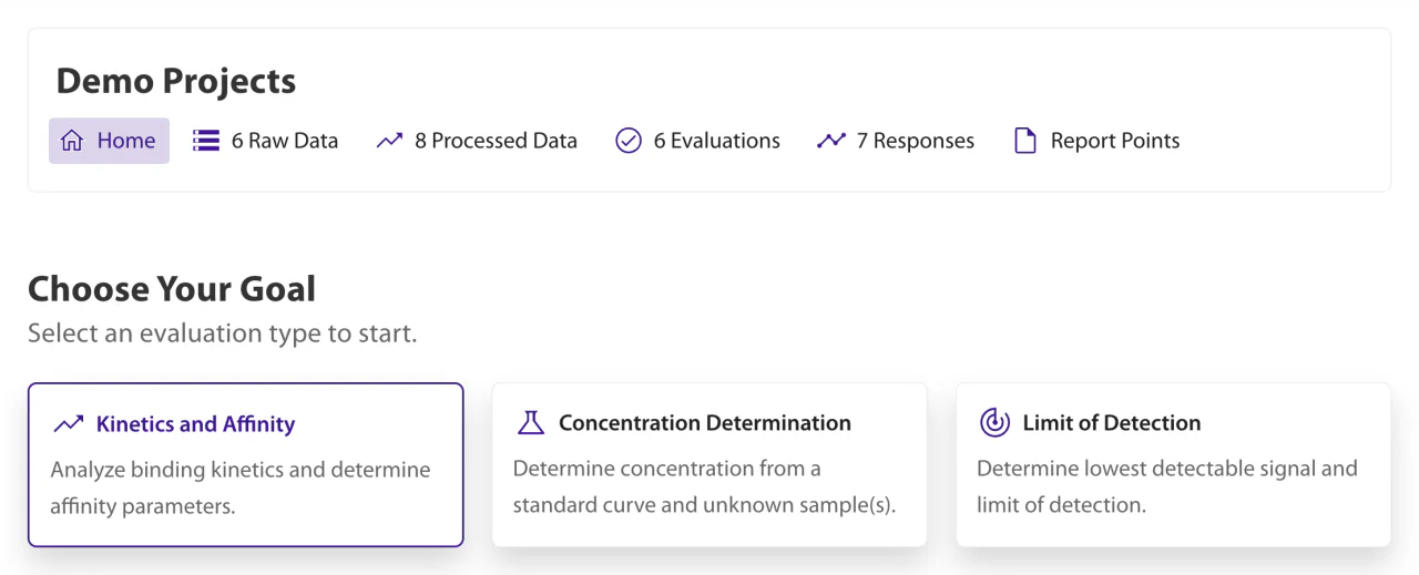
Each card leads to one evaluation. Evaluations compares the five by the data each one needs and the result it produces; the pages behind that table own the method. Below is the sequence they all share.
Run the workflow
- Select eligible raw data, processed data, or a previous evaluation in Data. Raw data can also be added to the project there.
- Review Cleanup when it is available. The listed actions are the data transformations the evaluation will use.
- Configure Parameters and, where available, inspect and accept fits in Fitting.
- Check the data, cleanup and settings in Review, then select Run.
Re-evaluate restores the previous data and settings in the same workflow and proposes a versioned name. Selecting an existing evaluation as input reuses its data and cleanup; fitting parameters return to the defaults for that data. See Data Cleanup for how to inspect and change those actions.
The Kinetics and Affinity wizard includes an Evaluation Assistant when the service is enabled. It can explain model choice, data requirements, cleanup and fit acceptance in the context of the current workflow.
Consensus Plot
With Advanced off, measurement plots use the default mologram selection for the chip and multiplexing. Custom mologram selections apply only in Advanced mode and are retained when you switch back to it. Downloads and cleanup inputs use the selection of the displayed plot.
Consensus Plot without Outliers
In Raw Data, enable Advanced, expand Plot controls & downloads, and select Consensus Plot without Outliers. The same plot is available under Data Selection when creating or editing processed data. Grouped injections use their dedicated group plot types instead.
The plot screens each multiplexing group independently for injection noise and inconsistent injection-end responses. Its line is a recorded trace from an accepted mologram, not a pointwise median. The legend shows how many molograms passed screening for each multiplexing group.
The shaded band describes the spread of accepted traces after they are aligned to the reference. It always contains the recorded reference where both are shown and is not a confidence interval. Rejected traces are hidden under one grey legend entry and can be revealed for shape comparison.
Screening uses the full measurement after cleanup actions are applied. Selecting a phase changes only the displayed interval. If the data cannot support screening, the plot shows a recorded reference without a band and labels it as insufficient screening data. This display does not remove sensors from stored data or downstream evaluations.
Compute Delta
Choose Compute Delta from Plot Actions and select Execute, then click two points on a live or completed measurement plot. The result dialog shows the time difference, value change, and slope for the clicked points together with mean, median, and standard deviation across the visible sensor traces represented by the plot. Traces that are hidden by default do not affect the calculation. Multi-trace data also includes 95% confidence intervals. A single-trace view still shows the statistics, using that trace as its sample. Mologram selection, normalization, and other displayed transformations are reflected in the calculation. Use Export CSV to download the summary and available per-trace values.
Working on Several Rows at Once
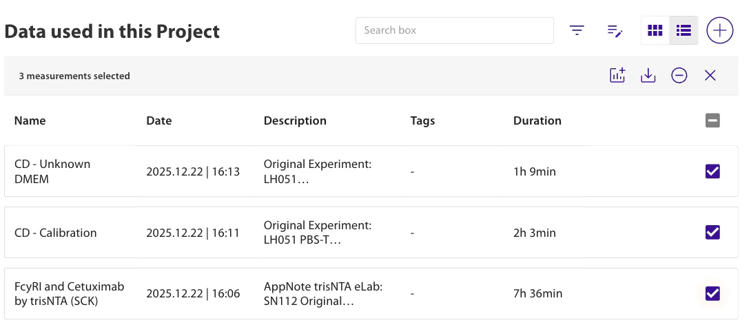
Turn on batch mode with the checkbox beside a table's filter — its tooltip reads Enable batch operations mode — to select rows and apply the actions shown above the table. (The Report Points table keeps its checkboxes on at all times.) Selections persist across pages but reset when the search, sort, or tag filter changes.
The available actions match the table — moving to a project, deleting, exporting, downloading, removing from a project, creating processed data, or plotting the selected rows. Failed rows remain selected for retry. A raw-data archive is created only when every selected measurement still has stored data.
The Projects list supports it too, in both its table and card views. Project table rows stay on the list while batch mode is active; use their checkboxes to select projects. Deleting projects asks once whether their processed data, evaluations, responses and report points go with them; measurements always stay. The project holding everything assigned to no other project cannot be selected.
Export measurement data
In measurement plots and Export Processed Data, use the download buttons beside the plot controls for interactive HTML or CSV files. Downloads save to your computer. The plot toolbar also offers PNG, Copy plot as PNG, and Download plot as SVG. SVG preserves the displayed curves, axes, labels, legend, and zoom range for reports and further editing.
| Action | Download |
|---|---|
| Download all CSV | A ZIP holding one folder per recorded quantity — coherent mass density and mass density — each with that quantity's metadata and timetraces, plus its injections and immobilizations where available. The export uses the processing algorithm preselected for the chip, or the first available one when the chip has no default. |
| Download raw data | The measurement database as recorded by the reader, with no processing applied. Each file takes the name of its measurement; several selected at once download together as one archive. |
Fit Timetraces
The Fit Timetraces tool interactively fits mathematical models to processed timetrace data, to characterize signal behavior or read off a rate constant. Open it from the Timetrace Fit action on a processed-data row.
- Specify: select the fit interval by Time Interval, Across Injections, or Multiple Injections and choose a fit function. Multiple Injections fits the selected injections together and excludes the data between them. Its percentage range selects the same portion of each injection. Optionally define a separate evaluation interval to display the fitted curve over a different range than the fit windows. Quality metrics describe the data used for fitting. Every selected fit window must contain recorded points for each mologram. Missing or invalid data in a fit window is reported as a failed fit for that mologram.
- Review: inspect per-sensor fit equations, parameters (with units), and quality metrics (R², RMSE, χ²ᵣ), then export the equations, parameters and plots. To subtract a fitted drift from the signal instead, use the Subtract fit cleanup action, which opens this same tool.
Supported fit functions: Linear, Quadratic, Exponential Decay and Double Exponential Decay (each with an optional baseline), and Exponential with Saturation (with an optional baseline).
The equation below the fit-function selector shows the parameters varied by the selected model and any parameter fixed at the start of the fit interval. Large timetraces are reduced to evenly spaced, plot-resolution input before fitting, and sensors are fitted concurrently.
Fitted drift: the fitting view spans the full measurement even when the processed-data selection is limited to one phase. The correction is still applied only to the selected data and successfully fitted molograms. It subtracts the change in the fitted curve relative to the start of the application interval, preserving the signal level at that boundary. For long-term linear drift removal, choose Multiple Injections, select a buffer at the beginning and one at the end, and choose Linear. The shaded windows in Review show the data used for fitting. Add an offset-removal action separately when the fitted signal should also be shifted to zero. Fitted drift is fitted against raw measurement data and must be the first cleanup action; the editor places a newly added fitted drift there automatically. A fitted-drift action is tied to the measurement, phase, property, and algorithm where its fit was created; create a new fit after changing any of them.