MACS Matchmaker
Every BIA experiment starts by attaching a ligand to the sensor surface. The choice of immobilization chemistry is not just a logistical detail — it shapes orientation, density, and stability. A heterogeneous-ligand fit may simply be telling you that random amine coupling produced a mix of orientations; a mass-transport-limited fit may be telling you the surface density is too high. On MACS Matchmaker sensors, almost every chemistry is presented through a DNA duplex (DDI), which decouples the ligand-attachment chemistry from the chip itself — even covalent NHS, maleimide, and click captures are regenerable as long as the duplex is the weakest link. The exception is direct on-chip click on the [Me-Tz|PEG] / [Me-Tz|Tz] sensors, where the ligand is covalently bound to the ridges and the chip is single-use per ligand.
How immobilization works
Immobilization is a flow step. The ligand is injected over the chip and binds the capture sites on the mologram ridges — on a DDI surface its oligo hybridises to the complementary ridge strand, on a click sensor it forms a covalent bond — and the instrument records the amount loaded as the immobilization level in pg/mm². The grooves are then filled with a non-binding probe matched to the ridge chemistry (backfilling) so the reference region cancels bulk and non-specific signal. The analyte binds this immobilized ligand in the injections that follow.
The recorded immobilization level carries through the analysis: it sets the expected Rmax, it is the reference the Normalize to immobilization cleanup action scales to, and its slow decay over a run is what a stability measurement fits.
Pick a chip and adapter
Three quick questions — sample matrix, ligand type, and throughput — map onto a concrete sensor + adapter combination from the lino portfolio. Use this as a starting point, then refine density and orientation choices using the sections below.
FM specifics: ridges, DDI, and click chemistry
A mologram interleaves ligand-bearing ridges with the reference grooves between them, so what matters is selective coupling to the activated ridges, not bulk surface coverage. lino achieves this in two ways. (1) DNA-Directed Immobilization (DDI): the chip carries a capture oligo on the ridges, and an oligo adapter brings the ligand in by hybridization — used for every Oligo|PEG and Oligo|Oligo sensor. (2) Direct click chemistry on the [Me-Tz|PEG] / [Me-Tz|Tz] sensors, where TCO-tagged ligands react bioorthogonally with the tetrazine-functionalized ridges via inverse-electron-demand Diels–Alder (TCO–Tz IEDDA), not the more common azide–alkyne click. TCO–Tz is copper-free, fast, and selective, but the bond is irreversible — the chip becomes single-use per ligand. Random orientation on the ridge surface still produces the heterogeneous-ligand pattern, so for kinetics use an oriented adapter (Protein A/G, trisNTA, Strep-Tactin XT, anti-GFP, Anti-Biotin) or a site-specifically TCO-tagged ligand whenever possible.
Common methods at a glance
The table compares the most common immobilization chemistries by orientation control, reversibility, and where each shines.
| Method | Chemistry | Orientation | Reversible? | Best for | Protocol |
|---|---|---|---|---|---|
| On-chip amine coupling (NHS oligo adapter) | A Me-Tz oligo adapter is hybridized first, a TCO–PEG–TFP linker clicks onto it on-chip, and the ligand primary amines then form a covalent amide with the TFP ester | Random | Yes — dehybridize the duplex to release ligand+adapter | Unmodified proteins or peptides; no off-chip conjugation step | NHS-adapter on-chip protocol |
| Off-chip amine DDI (AminoLink kit) | Lysines conjugated to an oligo off-chip with the AminoLink kit, then hybridized | Random | Yes — strip the duplex between ligands | Reusable chip for multi-ligand panels; tighter control over conjugate stoichiometry | AminoLink DDI protocol |
| Off-chip thiol DDI (ThioLink kit) | Maleimide oligo coupled to a free / engineered cysteine, then hybridized | Semi-controlled | Yes — strip the duplex | Ligands with one accessible Cys; more reproducible orientation than amine coupling | ThioLink DDI protocol |
| DEL hit splint ligation (5′-phosphate adapter) | T4 DNA Ligase joins the DEL hit’s 3′-OH tag to a 5′-phosphorylated chip-binding adapter via a splint oligo; the adapter then hybridizes onto the chip | DNA-tethered (compound at distal end of dsDNA tag) | Yes — strip the duplex | On-DNA DEL hit validation without re-synthesis; multiplex up to 64 compounds per chip | DEL splint-ligation protocol |
| Biotin capture | An oligo adapter captures a biotinylated ligand. The default adapter is a monovalent anti-biotin binder — reversible capture, one biotin per event, and the dissociation needed to keep backfilled grooves matched | Site-specific via biotin tag | Yes with the default dissociable adapter — duplex strip, or mild elution of the adapter–biotin complex | Biotinylated ligands, including on backfilled chips where the capture must stay dissociable and groove-matched | Anti-Biotin biotin-capture protocol |
| Anti-tag capture (Protein A/G, trisNTA, Strep-Tactin XT, anti-GFP) | Capture ligand pre-loaded on the chip via its oligo adapter, then flow tagged ligand | Oriented | Yes — both via tag elution and via duplex strip | Tagged recombinants (His, Strep, GFP-fusion) and IgGs; reuse the chip across many ligands | Anti-tag capture protocol |
| Fc-receptor capture (FcγRs, FcRn) | Pre-conjugated FcγR / FcRn–oligo adapter (catalogue) hybridizes to the chip; antibody flowed as analyte | Site-directed receptor presentation; antibody remains in solution | Yes — duplex strip | Fc-effector profiling across FcγRI / IIa / IIb / IIIa / IIIb and IgG PK / half-life screening (FcRn) | Fc-receptor capture protocol |
| Off-chip TCO–tetrazine click (DDI) | TCO oligo adapter clicks to a tetrazine-tagged ligand, then hybridizes | Site-specific if tagged off-chip | Yes — duplex strip | Custom-tagged ligands where you still want a regenerable surface | No step-by-step here — follow the instructions supplied with the oligo adapter you use. |
| On-chip TCO–tetrazine click (Sensor [Me-Tz|PEG] / [Me-Tz|Tz]) | Bioorthogonal IEDDA between TCO-tagged ligand and Me-Tz ridges — direct, no DDI | Site-specific if tagged off-chip | No — chip is single-use per ligand | Long-lived covalent attachment; lowest-cost sensor | TCO activation protocol |
Orientation matters for kinetics
Random covalent attachment (NHS lysine coupling, AminoLink DDI) exposes binding sites in a mix of orientations — some accessible, some occluded — and can show up as heterogeneous-ligand kinetics with two relaxation timescales (see Density tradeoffs for what that looks like in the trace). Oriented capture via the lino adapters (Protein A/G or Fc receptors for IgGs, trisNTA for His-tagged proteins, Strep-Tactin XT for Strep-tag II, anti-GFP VHH for GFP-fusions, Anti-Biotin for biotinylated ligands) usually reduces that heterogeneity and preserves binding-site accessibility better than random lysine coupling. It does not guarantee a homogeneous surface — conformation, loading and local environment still vary — so fit residuals and replicate behavior still have to be inspected.
Density tradeoffs
High ligand density gives more signal but invites mass-transport limitation (analyte gets consumed faster than it diffuses in) and rebinding (released analyte reattaches before leaving the boundary layer); see Ligand surface density for how this shapes the apparent kinetics. Choose the lowest ligand density that still gives a reproducible response across the concentration range you need. Estimate the response to aim for from the molecular-weight ratio and the expected active fraction, then confirm it experimentally against response, residuals and flow-rate dependence. Where a validated capture-level range exists for the chip and assay, use it. Equilibrium titrations tolerate higher density than kinetics.
On a DDI sensor the density is set by what you load, not only by how long you load it. Mixing the ligand-carrying adapter with unfunctionalized complementary DNA — the same strand without a ligand on it — fills part of the ridge with capture sites that cannot bind analyte, so the active density falls with the mixing ratio while the surface chemistry, and therefore the groove match, stays exactly the same. That makes the ratio a cleaner density control than shortening the immobilization, which leaves unhybridized capture strands behind instead.
one population, one decay rate — the fit the models assume
two ligand populations: a fast decay that stalls into a slow tail
rebinding flattens the decay and the off-rate reads far too slow
How do I measure immobilization stability?
Use the dissociation half-life, , to quantify immobilization stability: it is the time required for half of the immobilized ligand to dissociate. Isolate the immobilization and the buffer on either side of it, remove the offset using the pre-immobilization buffer, then fit the dissociation with Timetrace Fit and read the half-life from the fitted parameters. The walkthrough below does this on a capture of FcγRI by a trisNTA adapter.
- Add the measurement containing the immobilization to a project. Under Raw Data, plot the measurement and confirm that it includes the buffer before immobilization, the immobilization injection, and the following dissociation buffer.
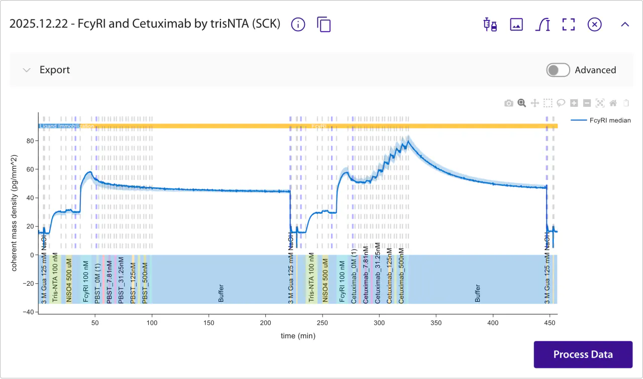
Plot the measurement containing the ligand immobilization. - Select Process Data, then choose Cut out → Keep only. Select Across Injections and set the range from the buffer before immobilization to the end of the buffer the ligand dissociates into. The half-life is read from that dissociation, so it has to be long enough to show one — here the run continues in buffer for about two hours.
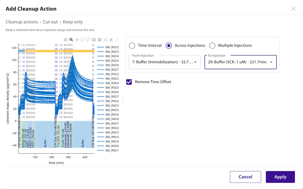
Keep the pre-immobilization buffer, the immobilization, and everything up to the end of the dissociation. - Add Offset → Remove offset from injection and select the first buffer injection. Apply the action, then save the processed data.
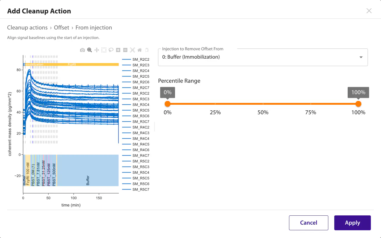
Use the first buffer injection as the known baseline. - Under Processed Data, open Timetrace Fit. For Fit Interval, select Across Injections and choose the long dissociation buffer for both From Injection and To Injection. Select Double Exponential Decay, then select Next.
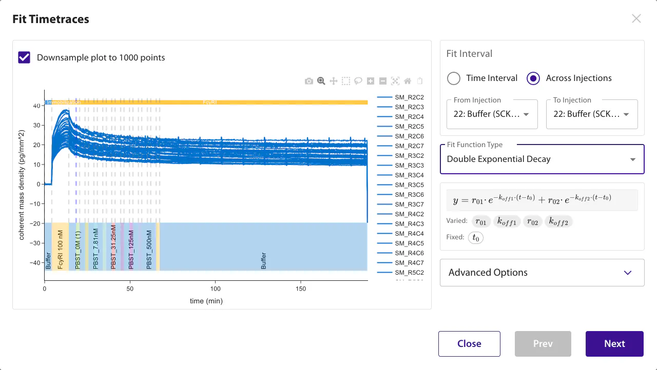
Fit the dissociation alone, with no baseline term to estimate. The baseline is known from the pre-immobilization buffer and was already removed, so the model without a baseline uses fewer free parameters. The double exponential represents the two dissociation processes suspected in this example. Use a single Exponential Decay when only one process is expected; a poor fit or systematic residuals can justify the double-exponential model.
- Review each sensor to confirm that the fit follows the trace and that the sensors behave consistently. Read and from the fitted parameters for the two dissociation processes. Sensors that fail to converge are named above the plot and excluded rather than forced; check that the failures are scattered rather than confined to one region of the chip, which would point at the surface instead of the fit.
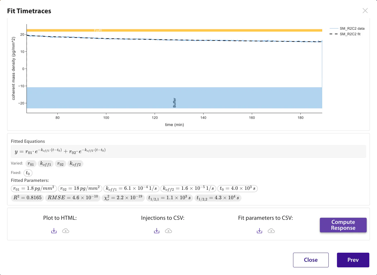
The fitted parameters report one half-life for each dissociation process.
Adapter choice and the reference region
A mologram references itself: ligand sits on the activated ridges and the grooves beside them are the reference region, so nothing is subtracted from a separate channel. Sub-micron self-referencing covers how that works. What it costs here is a constraint on which adapters can be used.
Where a no-ligand mologram is still useful is as a chemistry control — confirming the adapter itself (e.g. trisNTA, Protein A/G, Anti-Biotin) does not bind your analyte. It is a chemistry and assay control rather than a mandatory subtraction channel. It is one of several controls a run can carry; see Controls and replication for the others and for how to place them on the chip.
On the backfill-capable [Oligo|Oligo] and [Me-Tz|Tz] sensors the grooves are not left inert — they are backfilled with a chemically matched, non-active molecule so that abundant matrix proteins meet similar ridge and groove surfaces and are strongly suppressed in the coherent signal (see Backfilling and NSB suppression). Only use an adapter for backfilling if its capture is dissociable; an irreversible capture leaves the ridge and groove chemistries unmatchable and the two regions mix. For biotinylated ligands this is why the dissociable Oligo Adapter Anti-Biotin is the default; follow the Anti-Biotin biotin-capture protocol.